train_df = pd.read_csv('playground-series-s5e5/train.csv', index_col='id')
test_df = pd.read_csv('playground-series-s5e5/test.csv', index_col='id')
original_df = pd.read_csv('playground-series-s5e5/calories.csv', index_col="User_ID")Basics of Exploratory Data Analysis
machine learning
python
kaggle
Loading the data
- This data is from the Playground series in Kaggle (Season 5, Episode 5)
- Calorie Prediction Competition
- We let the
idcolumn in csv files to be the indexes in the dataframe, else it would have become an additional and unnecessary feature to handle
test_df.head()| Sex | Age | Height | Weight | Duration | Heart_Rate | Body_Temp | |
|---|---|---|---|---|---|---|---|
| id | |||||||
| 750000 | male | 45 | 177.0 | 81.0 | 7.0 | 87.0 | 39.8 |
| 750001 | male | 26 | 200.0 | 97.0 | 20.0 | 101.0 | 40.5 |
| 750002 | female | 29 | 188.0 | 85.0 | 16.0 | 102.0 | 40.4 |
| 750003 | female | 39 | 172.0 | 73.0 | 20.0 | 107.0 | 40.6 |
| 750004 | female | 30 | 173.0 | 67.0 | 16.0 | 94.0 | 40.5 |
Understanding the data
- Below we check if any
MissingorNaNvalues present in either ‘train’, ‘test’, ‘original’ data
# train_df.isna().sum().eq(0).all()
print((train_df.isna().sum() == 0).all())
print((test_df.isna().sum() == 0).all())
True
True- Getting information on all features in the data, particularly we can find which columns are numerical and which are not
- We identify that by looking at the
Dtypefor each columnObject: Categorical / text or stringfloat/int: is numerical, discrete or continuous
- This data looks fairly straight forward, as mostly the features seem numerical
- Only
Sexfeature is categorical, but that is also easy to handle as it has only 2 unique values
- We identify that by looking at the
- The stats of all numerical columns in train & test data look similar
- If you try comparing any statistic for a column in both train & test, they are very close
- So we can think of these data coming in from same distribution
print(train_df.describe().T)
print('--- ' * 20)
print('--- ' * 20)
print(test_df.describe().T)
count mean std min 25% 50% 75% max
Age 750000.0 41.420404 15.175049 20.0 28.0 40.0 52.0 79.0
Height 750000.0 174.697685 12.824496 126.0 164.0 174.0 185.0 222.0
Weight 750000.0 75.145668 13.982704 36.0 63.0 74.0 87.0 132.0
Duration 750000.0 15.421015 8.354095 1.0 8.0 15.0 23.0 30.0
Heart_Rate 750000.0 95.483995 9.449845 67.0 88.0 95.0 103.0 128.0
Body_Temp 750000.0 40.036253 0.779875 37.1 39.6 40.3 40.7 41.5
Calories 750000.0 88.282781 62.395349 1.0 34.0 77.0 136.0 314.0
--- --- --- --- --- --- --- --- --- --- --- --- --- --- --- --- --- --- --- ---
--- --- --- --- --- --- --- --- --- --- --- --- --- --- --- --- --- --- --- ---
count mean std min 25% 50% 75% max
Age 250000.0 41.452464 15.177769 20.0 28.0 40.0 52.0 79.0
Height 250000.0 174.725624 12.822039 127.0 164.0 174.0 185.0 219.0
Weight 250000.0 75.147712 13.979513 39.0 63.0 74.0 87.0 126.0
Duration 250000.0 15.415428 8.349133 1.0 8.0 15.0 23.0 30.0
Heart_Rate 250000.0 95.479084 9.450161 67.0 88.0 95.0 103.0 128.0
Body_Temp 250000.0 40.036093 0.778448 37.1 39.6 40.3 40.6 41.5- Get column names seperated into numerical & categorical categories
numerical_columns = [col for col in train_df.columns if train_df[col].dtype != 'object']
categorical_columns = [col for col in train_df.columns if train_df[col].dtype == 'object']
Univariate analysis: Plotting the data
1. Plot the categorical features, observations from below plots:
- Well balanced male / female classes in the train data
- When plotting box-plt of sex vs calories; min/max, all quartiles are located similarly for both male and female classes. Although there are a few more outliers calories in male class as compared to female class.
for col in categorical_columns:
    plt.figure(figsize=(12,6))

    plt.subplot(1,2,1)
    sns.boxplot(x=train_df[col], y=train_df['Calories'])

    plt.subplot(1,2,2)
    counts = train_df[col].value_counts()
    plt.pie(counts, labels=counts.index, autopct='%1.1f%%')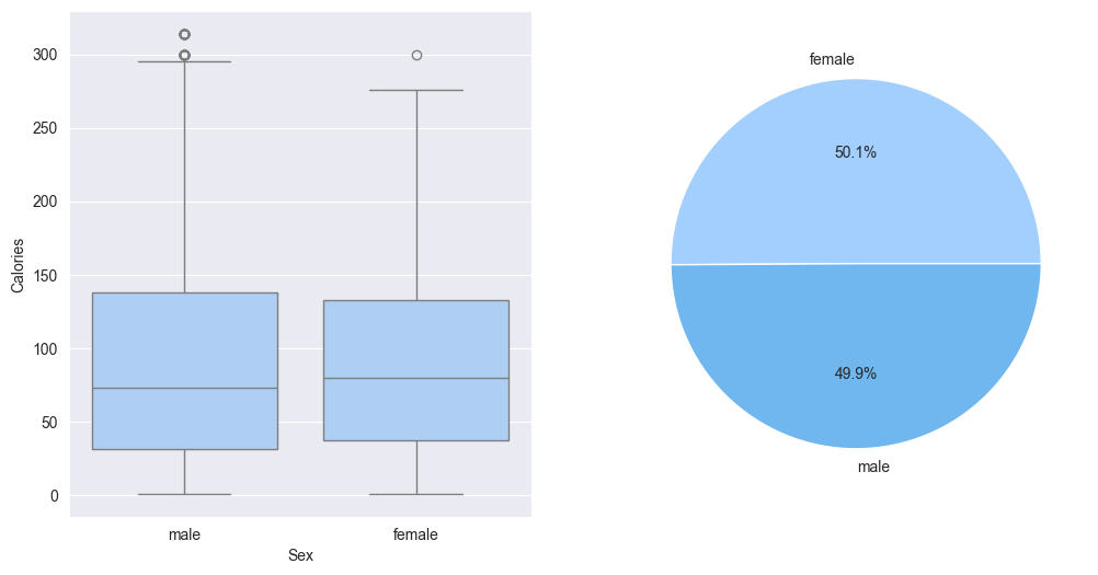
train_df[numerical_columns].skew()Age 0.436397
Height 0.051777
Weight 0.211194
Duration 0.026259
Heart_Rate -0.005668
Body_Temp -1.022361
Calories 0.539196
dtype: float64
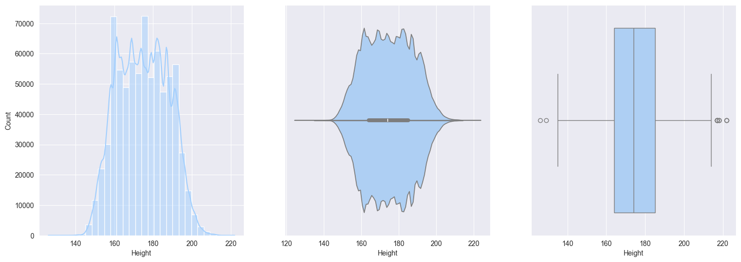
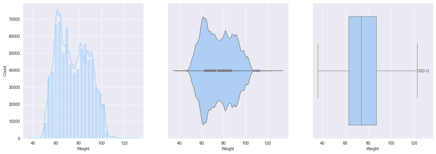
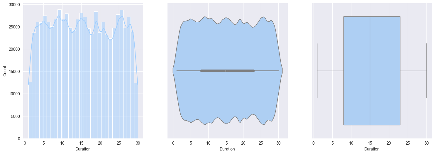
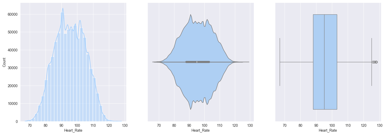
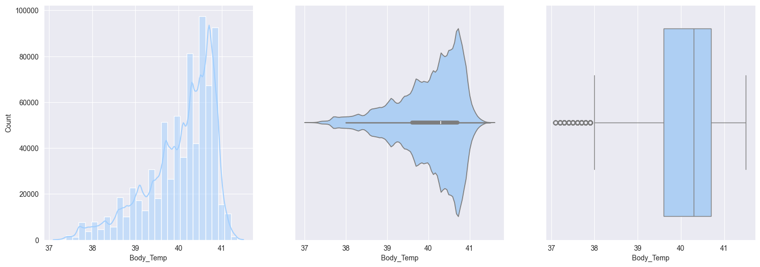
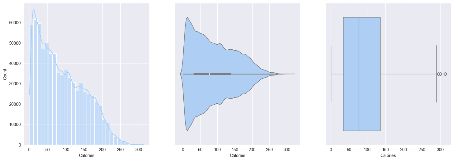
2. Plotting and observe the numerical features:
Age:- heavily skewed to right
- frequency decrease with increase in age
- may suggest that mostly younger people using the workout monitoring app
Height:- minimal skew
- symmetrical, bell shaped, approximately Gaussian (Normal) distribution
Weight:- slightly right skewed, which represent real-world data, upper limits can vary for wegihts
Duration:- approximately Uniform distribution
Heart_rate:- Normally distributed with slight righ skew
- small portion of people with elevated heart rates
Body_temp:- Negatively skewed
- after workout, slightly elevated from normal temperatures makes sense
Calories:- Right skewed, most people burn fewer calories per session, small fraction burn significantly more
for col in numerical_columns:
    plt.figure(figsize=(18,6))

    plt.subplot(1,3,1)
    sns.histplot(data=train_df[col], bins=30, kde=True)

    plt.subplot(1,3,2)
    sns.violinplot(x=train_df[col])

    plt.subplot(1,3,3)
    sns.boxplot(data=train_df[col], orient='h')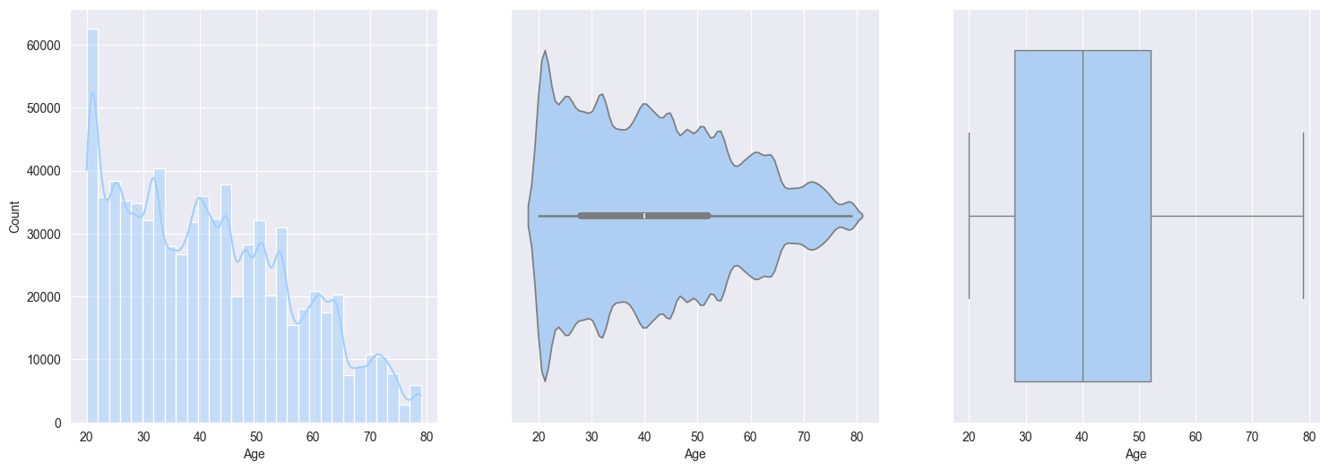
Bivariate analysis
- Let’s find the Correlations between the numerical features
# train_df[numerical_columns].corr().style.background_gradient()
corr = train_df[numerical_columns].corr()
# Plot the correlation matrix with colors
# Generate a mask for the upper triangle
mask = np.triu(np.ones_like(corr, dtype=bool))
# Set up the matplotlib figure
plt.figure(figsize=(5, 10))
# Generate a custom diverging colormap
cmap = sns.diverging_palette(230, 20, as_cmap=True)
# Draw the heatmap with the mask and correct aspect ratio
sns.heatmap(corr, mask=mask, cmap=cmap, vmax=.3, center=0,
square=True, linewidths=.5, cbar_kws={"shrink": .5}, annot=True)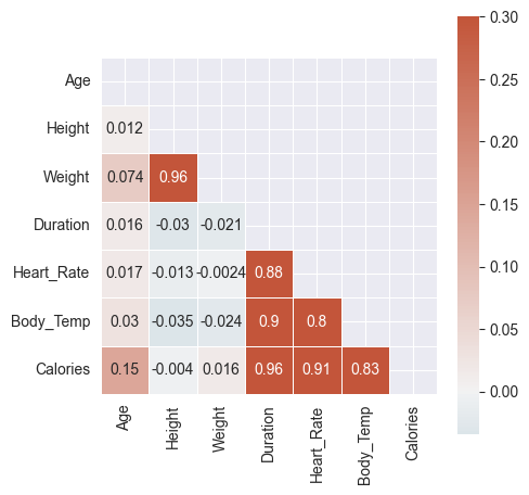
- Quite clear from above color gradients:
Caloriesis highly correlated withDuration,Heart_Rate,Body_TempHeart_RateandBody_Tempare highly correlatedDurationandHeart_Rateare highly correlatedDurationandBody_Tempare highly correlated
- Scatter plots amongst the numerical features
- Hardly any patterns emerge when we compare
CaloriestoAge,Weight,Height - Whereas, strong patterns can be seen with
Duration,Heart_Rate,Body_Temp
- Hardly any patterns emerge when we compare
So it’s fair to say that scatter plots confirm the correlation numbers
fig, axes = plt.subplots(2, 3, figsize=(18, 10))
axes = axes.ravel()  # Flatten the 2D array of axes for easy iteration

target = 'Calories'
for i, feature in enumerate(numerical_columns[:-1]):
    axes[i].scatter(train_df[feature], train_df[target], alpha=0.2)
    axes[i].set_xlabel(feature)
    axes[i].set_ylabel(target)
    axes[i].set_title(f'{feature} vs {target}')

plt.tight_layout()
plt.show()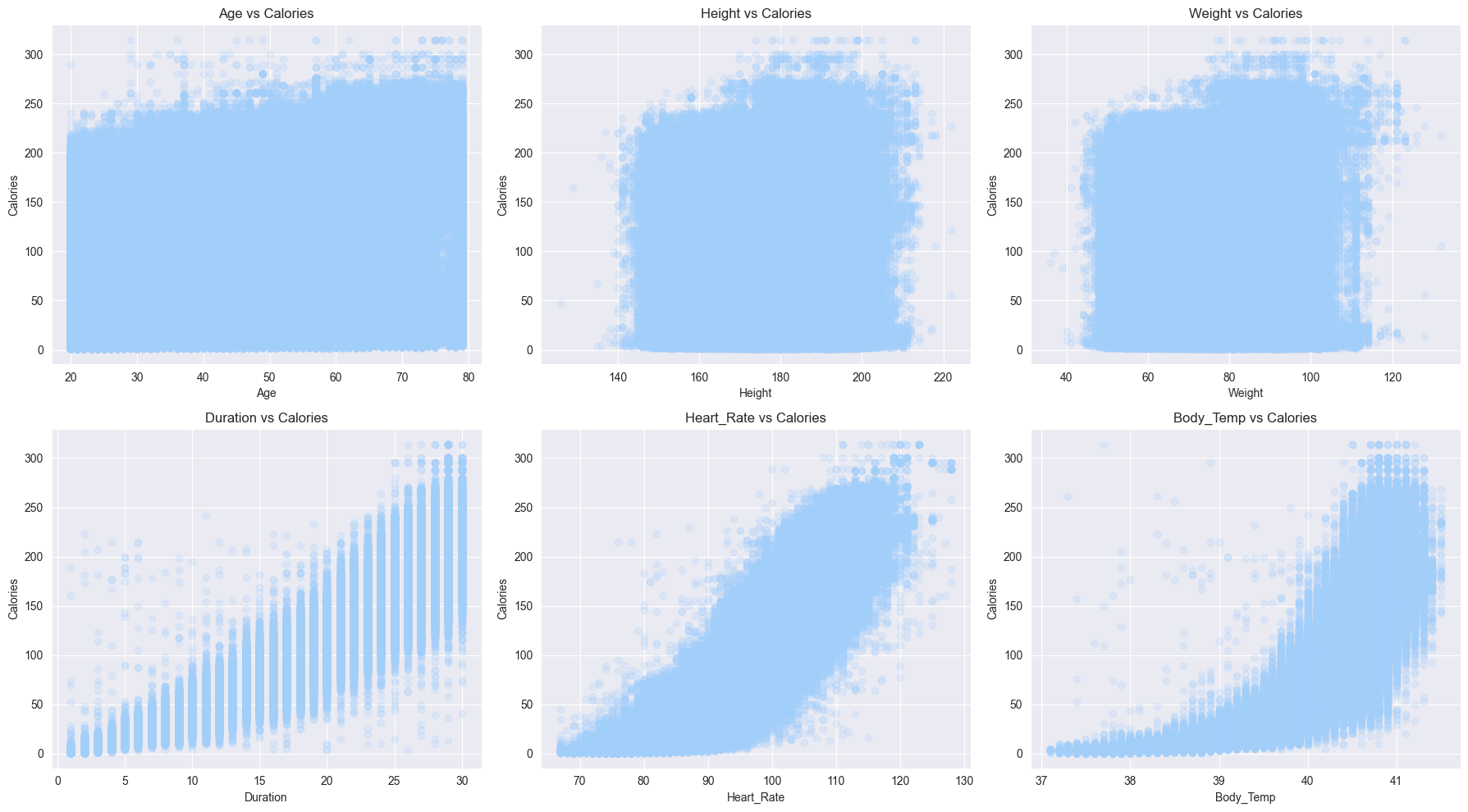
Data preprocessing
- Map the
Sexfeature into numerical
train_df['Sex'] = train_df['Sex'].map({'male':0, 'female':1})
test_df['Sex'] = test_df['Sex'].map({'male':0, 'female':1})- Make
Xandyvariables
X = train_df.drop('Calories', axis=1)
y = np.log1p(train_df['Calories'])
y_scale = (train_df['Calories'] - train_df['Calories'].mean()) / train_df['Calories'].std()
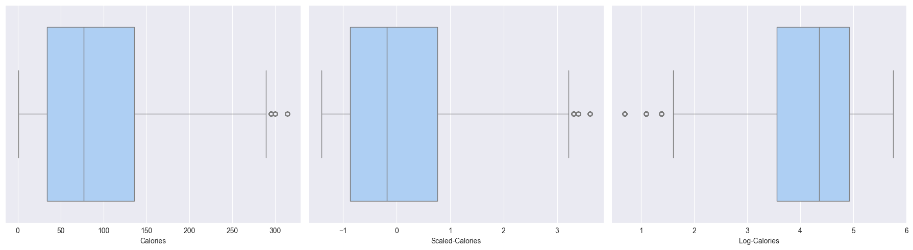
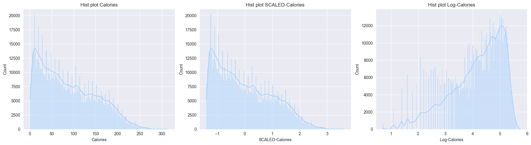
X_test = test_df- Now let’s try to differentiate between log transformation (
y) and standard scaled (y_scale)- Observations from the boxplots and histplots below:
- Scaling just scales the feature, but the distributions remains same, skew remains the same, outliers are still outliers
- Log transform changes the distribution by reducing the skew, also outliers are compressed
- Observations from the boxplots and histplots below:
# renaming Gender in original_df to Sex

original_df['Gender'] = original_df['Gender'].map({'male':0, 'female':1})
original_df = original_df.rename(columns={'Gender': 'Sex'})- As now we have original_df with same column names and no null samples, we can merge the train_df with original_df
# merge the original data to train_df
train_df = pd.concat([train_df, original_df])- This way we can get the Mutual Information scores of every feature in
Xagainsty(target)
from sklearn.feature_selection import mutual_info_regression
mi = mutual_info_regression(X=X, y=y, n_neighbors=5)
mutual_info = pd.Series(mi)
mutual_info.index = X.columns- The results of mututal_info_regression clearly concurs the scatter plot patterns and correlations
Duration,Heart_Rate,Body_Tempare containing most mutual information with the Calories- But, then, by human understanding,
Durationalso positively impacts bothHeart_Rate&Body_Temp
mutual_info = pd.DataFrame(mutual_info.sort_values(ascending=False), columns=['Mutual Information'])
mutual_info| Mutual Information | |
|---|---|
| Duration | 1.641538 |
| Body_Temp | 1.122338 |
| Heart_Rate | 0.977394 |
| Age | 0.098674 |
| Weight | 0.055857 |
| Height | 0.054949 |
| Sex | 0.016582 |
- Split the merged df, into train, dev, test split
# shuffle
train_df = train_df.sample(frac=1)
def scale_numerical_feature(X):
return (X - np.mean(X, axis=0)) / np.std(X, axis=0)Basic models
Simple Linear regression
- Using just most informative of the features
- I want to see how using just `Duration` would predict the `Calories`
class SimpleLinearRegression:
def __init__(self):
self.w = np.random.rand() * 0.01
self.b = np.random.rand() * 0
def get_params(self):
return (self.w, self.b)
# compute predictions for the given input X
def predict(self, X):
return (self.w * X + self.b)
def fit(self, X, y, epochs=100, lr = 0.01):
n = len(X)
for epoch in range(epochs):
# calculate prediction for X
y_pred = self.predict(X)
# calculate loss wrt y
loss = np.sqrt(np.mean((y_pred - y) ** 2))
# calculate gradients
dw = (2/n) * np.sum((y_pred - y) * X)
db = (2/n) * np.sum(y_pred - y)
# update the params
self.w -= lr * dw
self.b -= lr * db
# print(f'loss={loss}')
if (epoch + 1) % 100 == 0 or epoch == 0:
print(f'Epoch {epoch + 1}: Loss {loss:.4f}')
def evaluate(self, X, y):
y_pred = self.predict(X)
mse = np.mean((y_pred - y) ** 2)
rmse = np.sqrt(mse)
y_pred = np.clip(y_pred, 0, None)
y = np.clip(y, 0, None)
log_pred = np.log1p(y_pred)
log_true = np.log1p(y)
rmsle = np.sqrt(np.mean((log_pred - log_true) ** 2))
print(f'rmse: {rmse:.4f} | rmsle: {rmsle:.4f}')
# return mse, rmse, rmslen1 = int(0.8 * len(train_df))
n2 = int(0.9 * len(train_df))
X = scale_numerical_feature(train_df['Heart_Rate'])
y = train_df['Calories']
# y = np.log1p(train_df['Calories'])
# as we use RMSLE eval metric, we must not be pre-transforming Calories with np.log1p
X_train, y_train = X.values[:n1], y.values[:n1]
X_dev, y_dev = X.values[n1:n2], y.values[n1:n2]
X_test, y_test = X.values[n2:], y.values[n2:]# naive baseline (based on mean value prediction)
y_baseline = np.full_like(y_test, y_train.mean())
rmse_baseline = np.sqrt(np.mean((y_baseline - y_test) ** 2))
rmsle_baseline = np.sqrt(np.mean((np.log1p(y_baseline) - np.log1p(y_test)) ** 2))
print(f'rmse-baseline: {rmse_baseline}')
print(f'rmsle-baseline: {rmsle_baseline}')
print(f'mean of y_train: {y_train.mean()}')rmse-baseline: 62.389940344734526
rmsle-baseline: 1.0252838505834856
mean of y_train: 88.2883545751634Above, rmse_baseline indicates –> predicting with mean will be off on average by 62.4 calories - Hence, we must target that our simplest model acheives rmse below this number
model_1 = SimpleLinearRegression()
model_1.fit(X_train, y_train, epochs=200, lr=0.1)
Epoch 1: Loss 108.1040
Epoch 100: Loss 26.0761
Epoch 200: Loss 26.0761# return mse, rmse, rmsle
model_1.evaluate(X_test, y_test)rmse: 26.0880 | rmsle: 0.7414RMSEandRMSLEboth have improved over the baseline numbersLet’s work on comparing our custom linear regression model with the standard Sklearn LR
from sklearn.linear_model import LinearRegressiondef evaluate(y_pred, y_true):
mse = np.mean((y_pred - y_true) ** 2)
rmse = np.sqrt(mse)
y_pred = np.clip(y_pred, 0, None)
y_true= np.clip(y_true, 0, None)
log_pred = np.log1p(y_pred)
log_true = np.log1p(y_true)
rmsle = np.sqrt(np.mean((log_pred - log_true) ** 2))
print(f'rmse: {rmse:.4f} | rmsle: {rmsle:.4f}')
# return rmse, rmslesk_model_1 = LinearRegression()
sk_model_1.fit(X_train.reshape(-1,1), y_train)LinearRegression()In a Jupyter environment, please rerun this cell to show the HTML representation or trust the notebook.
On GitHub, the HTML representation is unable to render, please try loading this page with nbviewer.org.
LinearRegression()
y_pred = sk_model_1.predict(X_test.reshape(-1,1))
evaluate(y_pred, y_test)
rmse: 26.0880 | rmsle: 0.7414print(f'Weight converged to, by sklearn model: {sk_model_1.coef_[0]}')
print(f'Weight converged to, by custom model: {model_1.get_params()[0]}')Weight converged to, by sklearn model: 56.67769001861729
Weight converged to, by custom model: 56.67769001861444print(f'bias converged to, by sklearn model: {sk_model_1.intercept_}')
print(f'bias converged to, by custom model: {model_1.get_params()[1]}')bias converged to, by sklearn model: 88.29586143576026
bias converged to, by custom model: 88.29586143576023print(f'weights reached at from two methods are same? {math.isclose(sk_model_1.coef_[0], model_1.get_params()[0])}')
print(f'biases reached at from two methods are same? {math.isclose(sk_model_1.intercept_, model_1.get_params()[1])}')weights reached at from two methods are same? True
biases reached at from two methods are same? True- Good to conclude that out custom LR reach at almost same
weightandbiasas sklearn LR
def r2_score(y_pred, y_true):
    # print(f'shapes: y_pred - {y_pred.shape} | y_true - {y_true.shape}')
    ss_total = np.sum((y_pred - np.mean(y_true)) ** 2)
    ss_res = np.sum((y_pred - y_true) ** 2)
    r2 = 1 - (ss_res / ss_total)
    # print(f'ss_total: {ss_total} | ss_res: {ss_res}')
    print(f'r2: {r2:.4f}')
    # return r2
y_pred_1 = model_1.predict(X_test)
y_pred_sk_1 = sk_model_1.predict(X_test.reshape(-1,1))
r2_score(y_pred_1, y_test), r2_score(y_pred_sk_1, y_test)r2: 0.7880
r2: 0.7880(None, None)- R-squared also is similar using both models: 78.8 %
Making it multivariate regression
class MultipleLinearRegression:
    def __init__(self, n_features):
        self.w = np.random.rand(n_features,) * 0.1
        self.b = np.random.rand() * 0.0

    def get_params(self):
        return (self.w, self.b)

    # compute predictions for the given input X
    def predict(self, X):
        # (n_samples, n_features) @ (n_features,)    --> (n_samples,)
        out = X @ self.w + self.b
        return out

    def fit(self, X, y, epochs=100, lr = 0.01):
        n = len(X)
        for epoch in range(epochs):
            # calculate prediction for X
            y_pred = self.predict(X)

            # calculate loss wrt y
            loss = np.sqrt(np.mean((y_pred - y)**2))

            # calculate gradients
            dw = (2/n) * np.dot(X.T, (y_pred - y)) # shape: (n_features,)
            db = (2/n) * np.sum(y_pred - y) # shape: scalar

            # update the params
            self.w -= lr * dw
            self.b -= lr * db

            # print(f'loss={loss}')
            if (epoch + 1) % 100 == 0 or epoch == 0:
                print(f'Epoch {epoch + 1}: Loss {loss:.4f}')

    def evaluate(self, X, y):
        y_pred = self.predict(X)

        mse = np.mean((y_pred - y) ** 2)
        rmse = np.sqrt(mse)

        # rmsle = np.sqrt(np.mean((np.log1p(y) - np.log1p(y_pred)) ** 2))
        y_pred = np.clip(y_pred, 0, None)
        y = np.clip(y, 0, None)
        log_pred = np.log1p(y_pred)
        log_true = np.log1p(y)
        rmsle = np.sqrt(np.mean((log_pred - log_true) ** 2))

        print(f'rmse: {rmse:.4f} | rmsle: {rmsle:.4f}')
        # return mse, rmse, rmsle
n_features = 2
X = scale_numerical_feature(train_df[['Duration', 'Heart_Rate']])
y = train_df['Calories']


X_train, y_train = X.values[:n1], y.values[:n1]
X_dev, y_dev = X.values[n1:n2], y.values[n1:n2]
X_test, y_test = X.values[n2:], y.values[n2:]
model_2 = MultipleLinearRegression(n_features=2)
model_2.fit(X_train, y_train, epochs=200, lr=0.5)Epoch 1: Loss 108.0551
Epoch 100: Loss 15.1002
Epoch 200: Loss 15.1002sk_model_2 = LinearRegression()
sk_model_2.fit(X_train, y_train)LinearRegression()In a Jupyter environment, please rerun this cell to show the HTML representation or trust the notebook.
On GitHub, the HTML representation is unable to render, please try loading this page with nbviewer.org.
LinearRegression()
print(f'Weight converged to, by sklearn model: {sk_model_2.coef_}')
print(f'Weight converged to, by custom model:   {model_2.get_params()[0]}')
Weight converged to, by sklearn model: [43.88145203 18.28755783]
Weight converged to, by custom model: [43.88145203 18.28755783]np.allclose(sk_model_2.intercept_, model_2.get_params()[1])True# return mse, rmse, rmsle
model_2.evaluate(X_test, y_test)rmse: 15.1551 | rmsle: 0.6282y_pred_2 = model_2.predict(X_test)
y_pred_sk_2 = sk_model_2.predict(X_test)
r2_score(y_pred_2, y_test), r2_score(y_pred_sk_2, y_test)r2: 0.9372
r2: 0.9372(None, None)n_features = 3
X = scale_numerical_feature(train_df[['Duration', 'Heart_Rate', 'Body_Temp']])
y = train_df['Calories']

X_train, y_train = X.values[:n1], y.values[:n1]
X_dev, y_dev = X.values[n1:n2], y.values[n1:n2]
X_test, y_test = X.values[n2:], y.values[n2:]%time
model_3 = MultipleLinearRegression(n_features=3)
model_3.fit(X_train, y_train, epochs=300, lr=0.1)CPU times: user 2 μs, sys: 1e+03 ns, total: 3 μs
Wall time: 3.81 μs
Epoch 1: Loss 108.0602
Epoch 100: Loss 14.2118
Epoch 200: Loss 13.9630
Epoch 300: Loss 13.9518sk_model_3 = LinearRegression()
sk_model_3.fit(X_train, y_train)LinearRegression()In a Jupyter environment, please rerun this cell to show the HTML representation or trust the notebook.
On GitHub, the HTML representation is unable to render, please try loading this page with nbviewer.org.
LinearRegression()
Weight converged to, by sklearn model: [ 55.76189897  18.59805859 -13.45353933]
Weight converged to, by custom model:   [ 55.41889798  18.73747023 -13.23810133]
np.allclose(sk_model_3.intercept_, model_3.get_params()[1])True# return mse, rmse, rmsle
model_3.evaluate(X_test, y_test)rmse: 13.9925 | rmsle: 0.5184y_pred_3 = model_3.predict(X_test)
y_pred_sk_3 = sk_model_3.predict(X_test)
r2_score(y_pred_3, y_test), r2_score(y_pred_sk_3, y_test)r2: 0.9469
r2: 0.9469(None, None)There is a clear improvement in the regression as it does increase the variability explained over mean prediction, by increase in number of features: - n_features = 1 | R-squared = 78.8 % - n_features = 2 | R-squared = 83.7 % - n_features = 3 | R-squared = 94.6 %
Implementing Mini-batch gradient descent
- For now we were only calculating loss over entire
X_trainat once and running gradient descent. - So let’s try to first break it up into mini-batches
- This will help us train and also converge faster hopefully
# training with mini-batch
class CustomLinearRegression:
    def __init__(self):
        self.w = None
        self.b = None

    def get_params(self):
        return (self.w, self.b)

    def predict(self, X):
        out = X @ self.w + self.b
        return out

    def compute_loss(self, y_pred, y):
        loss = np.sqrt(np.mean((y_pred - y)**2))
        return loss

    def compute_gradients(self, X, y, y_pred):
        n = len(y)
        dw = (2/n) * np.dot(X.T, (y_pred - y)) # shape: (n_features,)
        db = (2/n) * np.sum(y_pred - y) # shape: scalar
        return dw, db

    def fit(self, X, y, epochs=100, batch_size = 128, lr = 0.01):
        n_samples, n_features = X.shape
        self.w = np.random.rand(n_features,) * 0.01
        self.b = np.random.rand() * 0.0

        for epoch in range(epochs):
            indexes = np.random.choice(a = n_samples, size = batch_size)
            Xb, yb = X[indexes], y[indexes]
            # print(Xb.shape, yb.shape)

            # calculate prediction for X
            y_pred = self.predict(Xb)

            # calculate loss wrt y
            loss = self.compute_loss(y_pred, yb)

            # calculate gradients
            dw, db = self.compute_gradients(Xb, yb, y_pred)

            # update the params
            self.w -= lr * dw
            self.b -= lr * db

            # print(f'loss={loss}')
            self.print_loss(loss, epoch)
            # if (epoch + 1) % 1000 == 0 or epoch == 0:
            #     print(f'Epoch {epoch + 1}: Loss {loss:.4f}')

    def print_loss(self, loss, epoch):
        if (epoch + 1) % 1000 == 0 or epoch == 0:
                print(f'Epoch {epoch + 1}: Loss {loss:.4f}')

    def evaluate(self, X, y):
        y_pred = self.predict(X)

        mse = np.mean((y_pred - y) ** 2)
        rmse = np.sqrt(mse)

        # rmsle = np.sqrt(np.mean((np.log1p(y) - np.log1p(y_pred)) ** 2))
        y_pred = np.clip(y_pred, 0, None)
        y = np.clip(y, 0, None)
        log_pred = np.log1p(y_pred)
        log_true = np.log1p(y)
        rmsle = np.sqrt(np.mean((log_pred - log_true) ** 2))

        print(f'rmse: {rmse:.4f} | rmsle: {rmsle:.4f}')
# return mse, rmse, rmsle%time
model_3_mb = CustomLinearRegression()
model_3_mb.fit(X_train, y_train, epochs=10000, batch_size=4096, lr=0.05)CPU times: user 3 μs, sys: 1e+03 ns, total: 4 μs
Wall time: 4.05 μs
Epoch 1: Loss 106.6047
Epoch 1000: Loss 13.9319
Epoch 2000: Loss 13.9302
Epoch 3000: Loss 13.7890
Epoch 4000: Loss 14.1124
Epoch 5000: Loss 14.4587
Epoch 6000: Loss 13.1583
Epoch 7000: Loss 14.1098
Epoch 8000: Loss 13.3162
Epoch 9000: Loss 13.8549
Epoch 10000: Loss 14.0191model_3_mb.evaluate(X_test, y_test)rmse: 13.9915 | rmsle: 0.5183y_pred_3_mb = model_3_mb.predict(X_test)
r2_score(y_pred_3_mb, y_test), r2_score(y_pred_sk_3, y_test)r2: 0.9470
r2: 0.9469(None, None)So, the mini-batch implementation is working, although - The results are not any better, probably it takes way faster to run a single update - Expectation is, when the data and model both become much more complex, the gains from using mini-batch must be visible
Regularization - L2 norm
class CustomLinearRegressionL2(CustomLinearRegression):

    def __init__(self, lambda_ = 0.1):
        super().__init__()
        self.lambda_ = lambda_

    def print_loss(self, loss, epoch):
        if (epoch + 1) % 10000 == 0 or epoch == 0:
                print(f'Epoch {epoch + 1}: Loss {loss:.4f}')

    def compute_loss(self, y_pred, y):
        rmse = np.sqrt(np.mean((y_pred - y) ** 2))
        l2_penalty = self.lambda_ * np.sum(self.w ** 2)
        loss = rmse + l2_penalty
        return loss

    def compute_gradients(self, X, y, y_pred):
        n = len(y)
        dw = (2/n) * np.dot(X.T, (y_pred - y)) + (2 * self.lambda_ * self.w)
        db = np.sum(y_pred - y)
        return dw, db
model_3_l2 = CustomLinearRegressionL2(lambda_=0.01)
model_3_l2.fit(X_train, y_train, epochs=20000, batch_size=1024, lr=1e-4)Epoch 1: Loss 111.0268
Epoch 10000: Loss 32.2485
Epoch 20000: Loss 31.9944model_3_l2.evaluate(X_test, y_test)rmse: 17.2014 | rmsle: 0.6512Using all features
numerical_columns.pop()
numerical_columns
['Age', 'Height', 'Weight', 'Duration', 'Heart_Rate', 'Body_Temp']# scaling all the numerical features
X = train_df.drop('Calories', axis=1)
X[numerical_columns] = scale_numerical_feature(X[numerical_columns])
y = train_df['Calories']
# y = np.log1p(train_df['Calories'])
X_train, y_train = X.values[:n1], y.values[:n1]
X_dev, y_dev = X.values[n1:n2], y.values[n1:n2]
X_test, y_test = X.values[n2:], y.values[n2:]model_l2_all = CustomLinearRegressionL2(lambda_=0.01)
model_l2_all.fit(X_train, y_train, epochs=20000, batch_size=4096, lr=1e-4)Epoch 1: Loss 107.9762
Epoch 10000: Loss 30.4919
Epoch 20000: Loss 30.5582model_l2_all.evaluate(X_dev, y_dev)rmse: 14.9929 | rmsle: 0.6459With using all of the features, we see there is improvement in R-squared (although small)
Test set predictions with our best model (as per rmsle)
# test_df.head()# # test_df[numerical_columns] = scale_numerical_feature(test_df[numerical_columns])
# X = scale_numerical_feature(test_df[['Duration', 'Heart_Rate', 'Body_Temp']])
# X_test = X.values
# # X.shape, test_df.shape
# ids = X.index# y_test_preds = model_3.predict(X_test)
# y_test_preds = np.clip(y_test_preds, 0, None)# import csv
# with open('submission_using_3features.csv', 'w') as f:
# writer = csv.writer(f)
# writer.writerow(['id', 'Calories'])
# writer.writerows(zip(ids.tolist(), y_test_preds.tolist()))Conclusion
After trying with multiple feature combinations (or even all features), to model the Calories:
- We notice that the
rmslemetric an order of magnitude larger than what mostly submissions show in the Kaggle competitions - Possibly, it’s because of the Heteroskedasticity in the data, i.e., the errors vary in different ranges of X.
- The basic assumption for Linear Regression to work is that data should have some linear relationaship.
- Therefore, for us to reach desired range of
rmsle, we shall pivot to more advanced algorithms.- XGBoost, CatBoost etc.